Blocker: Random Effects Meta-Analysis of Clinical Trials¶

An example from OpenBUGS [38] and Carlin [13] concerning a meta-analysis of 22 clinical trials to prevent mortality after myocardial infarction.

Model¶

Events are modelled as

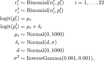
$r^c_i &\sim \text{Binomial}(n^c_i, p^c_i) \quad\quad i=1,\ldots,22 \\ r^t_i &\sim \text{Binomial}(n^t_i, p^t_i) \\ \operatorname{logit}(p^c_i) &= \mu_i \\ \operatorname{logit}(p^t_i) &= \mu_i + \delta_i \\ \mu_i &\sim \text{Normal}(0, 1000) \\ \delta_i &\sim \text{Normal}(d, \sigma) \\ d &\sim \text{Normal}(0, 1000) \\ \sigma^2 &\sim \text{InverseGamma}(0.001, 0.001),$

where $r^c_i$ is the number of control group events, out of $n^c_i$ , in study $i$ ; and $r^t_i$ is the number of treatment group events.

Analysis Program¶

using Mamba

## Data
blocker = (Symbol => Any)[
  :rt =>
    [3, 7, 5, 102, 28, 4, 98, 60, 25, 138, 64, 45, 9, 57, 25, 33, 28, 8, 6, 32,
     27, 22],
  :nt =>
    [38, 114, 69, 1533, 355, 59, 945, 632, 278, 1916, 873, 263, 291, 858, 154,
     207, 251, 151, 174, 209, 391, 680],
  :rc =>
    [3, 14, 11, 127, 27, 6, 152, 48, 37, 188, 52, 47, 16, 45, 31, 38, 12, 6, 3,
     40, 43, 39],
  :nc =>
    [39, 116, 93, 1520, 365, 52, 939, 471, 282, 1921, 583, 266, 293, 883, 147,
     213, 122, 154, 134, 218, 364, 674]
]
blocker[:N] = length(blocker[:rt])


## Model Specification

model = Model(

  rc = Stochastic(1,
    @modelexpr(mu, nc, N,
      begin
        pc = invlogit(mu)
        Distribution[Binomial(nc[i], pc[i]) for i in 1:N]
      end
    ),
    false
  ),

  rt = Stochastic(1,
    @modelexpr(mu, delta, nt, N,
      begin
        pt = invlogit(mu + delta)
        Distribution[Binomial(nt[i], pt[i]) for i in 1:N]
      end
    ),
    false
  ),

  mu = Stochastic(1,
    :(Normal(0, 1000)),
    false
  ),

  delta = Stochastic(1,
    @modelexpr(d, s2,
      Normal(d, sqrt(s2))
    ),
    false
  ),

  delta_new = Stochastic(
    @modelexpr(d, s2,
      Normal(d, sqrt(s2))
    )
  ),

  d = Stochastic(
    :(Normal(0, 1000))
  ),

  s2 = Stochastic(
    :(InverseGamma(0.001, 0.001))
  )

)


## Initial Values
inits = [
  [:rc => blocker[:rc], :rt => blocker[:rt], :d => 0, :delta_new => 0,
   :s2 => 1, :mu => zeros(blocker[:N]), :delta => zeros(blocker[:N])],
  [:rc => blocker[:rc], :rt => blocker[:rt], :d => 2, :delta_new => 2,
   :s2 => 10, :mu => fill(2, blocker[:N]), :delta => fill(2, blocker[:N])]
]


## Sampling Scheme
scheme = [AMWG([:mu], fill(0.1, blocker[:N])),
          AMWG([:delta, :delta_new], fill(0.1, blocker[:N] + 1)),
          Slice([:d, :s2], [1.0, 1.0])]
setsamplers!(model, scheme)


## MCMC Simulations
sim = mcmc(model, blocker, inits, 10000, burnin=2500, thin=2, chains=2)
describe(sim)

Results¶

Iterations = 2502:10000
Thinning interval = 2
Chains = 1,2
Samples per chain = 3750

Empirical Posterior Estimates:
              Mean        SD       Naive SE       MCSE         ESS
delta_new -0.25005767 0.15032528 0.0017358068 0.0042970294 1223.84778
       s2  0.01822186 0.02112127 0.0002438874 0.0012497271  285.63372
        d -0.25563567 0.06184194 0.0007140893 0.0030457284  412.27207

Quantiles:
              2.5%       25.0%       50.0%       75.0%       97.5%
delta_new -0.53854055 -0.32799584 -0.25578493 -0.17758841  0.07986060
       s2  0.00068555  0.00416488  0.01076157  0.02444208  0.07735715
        d -0.37341230 -0.29591698 -0.25818488 -0.21834138 -0.12842580